Wagner's Birthday Attack - How to Break InsecureMuSig

Introduction

MuSig is a protocol which allows mutually distrustful parties to safely create aggregated digital signatures together. I highly recommend you read my MuSig article before diving into this one, as it lays down the context. If you’re already familiar with MuSig and Schnorr, carry on!

The MuSig protocol has several iterations:

1. InsecureMuSig - An outdated and insecure 2-round version
2. MuSig1 - The secure 3-round variant
3. MuSig2 - The faster but slightly less secure 2-round variant

InsecureMuSig - the original form of MuSig - was proven insecure by Drijvers et al in 2018. The attack described in their paper depended on the fact that under InsecureMuSig, co-signers could manipulate the final aggregated nonce used for signing by submitting rogue nonces, computed as a function of their peers’ nonces. In response, the authors of MuSig amended their paper with a third nonce-commitment round of communication, thus preventing co-signers from providing rogue nonces.

This Blockstream article briefly summarizes the approach used by the attack, but only from the perspective an attack on an insecure implementation of MuSig1, in which nonces themselves are pre-shared before the message to sign is chosen. For a time, this article led me to mistakenly assume that it was the pre-sharing of nonces which made InsecureMuSig so insecure. However, that is not the approach used by Drijvers et al in their original paper. In the paper, Drijvers et al made no mention of nonce pre-sharing at all.

To my knowledge, there does not yet exist a full approachable explanation of how Wagner’s Attack broke InsecureMuSig. That is what I hope this article will be.

Bear in mind that I am no expert on Wagner’s Algorithm, but merely a tourist inclined to investigate algorithms which I find interesting. If you notice any mistakes, please suggest an edit on Github, or email me! I’d be very grateful for the help.

Notation

Just so we’re all on the same page:

Notation	Meaning
	The value is a member of set .
	The sum of all from to . i.e.
	is equivalent to modulo .
	The base-point of the secp256k1 curve.
	The order of the secp256k1 curve. There are possible valid non-zero points on the curve, plus the ‘infinity’ point (AKA zero).
	A cryptographically secure namespaced hash function under the namespace . Returns an integer mod .
	Sampling randomly from the set of integers modulo . Note that we exclude zero when sampling.
	Sampling randomly from the set of secp256k1 curve points. Note that we exclude the point at infinity (AKA zero) when sampling.
	Concatenation of the byte arrays and .
	The set of all integers from to (inclusive), i.e. every such that
	“For every element in set .”
	The order of (AKA number of elements in) set .

The Attack

The Setup

Alice, Bob and Carol have an aggregated public key defined as per the normal MuSig1 protocol.

Carol has some evil message she wants to sign using the aggregated key, but which Alice and Bob would never agree to sign. Perhaps a signature on would steal all of Alice and Bob’s Bitcoins. Perhaps it would sign a TLS certificate which only Carol shouldn’t actually have. Perhaps it is the string “Alice sucks and must not be invited to parties”. You get the idea.

Requirements

Carol will execute her dastardly attack by opening a number of concurrent signing sessions with Alice and Bob, and providing a set of carefully chosen rogue nonces. Rogue nonces behave similarly to rogue keys, which I highlighted in my MuSig article. If Carol learns Alice’s nonce and Bob’s nonce before revealing her own nonce , then Carol can offer up a rogue nonce which fools Alice and Bob into computing the aggregated nonce to be whatever Carol desires. When Carol does this, she can cause Alice and Bob’s signatures on to change in a way she fully controls, albeit unpredictably.

The “fully controls” part is particularly important. For Wagner’s Attack to work Carol must learn Alice and Bob’s public nonces before choosing her own, otherwise she cannot control the challenge and her attack will not work.

This is why InsecureMuSig was insecure: Unlike MuSig1, InsecureMuSig didn’t have a nonce-commitment phase. Co-signers simply exchanged their public nonces at will with no additional commitment phase or scrambling involved.

The Procedure

OK enough babbling. Let’s dive right in and see how Carol attacks this system.

1. Carol opens concurrent signing sessions with Alice and Bob, in which she proposes to sign innocuous messages which Alice and Bob would be perfectly agreeable to signing. can be any power of two - higher is generally more efficient, but riskier for Carol. should approach but not exceed the maximum number of concurrent signing sessions that Alice and Bob can safely handle.

2. Carol waits for Alice and Bob to share their public nonces with her in every one of the signing sessions.

3. Carol picks a nonce of her own which will protect her private key once the forgery is complete.

4. Carol runs Wagner’s Algorithm to find different curve points which hash to challenges which sum to an evil challenge .

• is the “evil nonce” which will eventually be used for Carol’s forged signature. It is the sum of all of Alice and Bob’s nonces across all signing sessions, plus Carol’s own nonce .
• Each is hashed with the message to produce a challenge for signing session .
• Through the wonder of Wagner’s Algorithm, the sum of all those hashes equals another hash which Carol has chosen based on an evil message (which Alice and Bob never see).

5. Carol calculates a set of rogue nonces , one for each signing session.

The purpose of each rogue nonce is to fool Alice and Bob into using the point as the aggregated nonces for signing session . Alice and Bob, upon receiving , will compute the aggregate nonce as:

Alice and Bob do not know to avoid . Because InsecureMuSig lacks nonce commitments, Alice and Bob do not know whether Carol provided a genuine nonce or a rogue one.

Carol can thus convince Alice and Bob to sign with the “aggregated” nonces chosen by Carol. She can do this because she waited for Alice and Bob to expose their nonces to her, so she can easily compute her nonces as a function of theirs.

By now, perhaps you are starting to see why why Carol needed to open those signing sessions concurrently (at the same time), rather than sequentially. She needs to know all of Alice and Bob’s nonces in order to compute the points with Wagner’s Algorithm, so she had to at least start the signing sessions before she could perform step 4. However, she also can’t conclude any signing session until she knows which point to aim for with her rogue nonce. Thus, the signing sessions must be concurrent.

6. Carol awaits the resulting pairs of partial signatures from Alice and Bob.

Let and denote Alice and Bob’s secret nonces for signing session . We can assume these are honestly random and unknown to Carol.

Alice and Bob will have computed their partial signatures as follows.

See how by selecting rogue nonces, Carol convinced her peers to sign the challenges which were selectively chosen by Carol, such that .

7. Carol sums Alice and Bob’s partial signatures from those signing sessions to create a usable forged signature which verifies under the aggregate key on Carol’s chosen message and evil nonce . Carol must add her own partial signature to complete the forgery.

This seems a bit too easy. How could this possibly work? Let’s expand to see why it would be valid.

_{Group the private nonces all on the left, Alice and Bob’s private key terms in the middle, and Carol’s private key term on the right.}

that doesn’t look like a valid Schnorr signature.

Not yet! But what if we…

Substitute All The Things

Here’s where the magic of Wagner’s Algorithm makes itself felt. Recall how Carol used Wagner’s Algorithm to find the the challenges so that they sum to her evil challenge .

_{Wondering how Carol did this? We’ll get there eventually.}

This relationship allows Carol to factor out from the aggregated partial signatures, just as with a regular aggregated Schnorr signature, except this time they are super-duper aggregated - a rigorous technical term which denotes that the signatures came from many signing sessions and from multiple peers.

Oh look. Now we can merge the middle and right groups of terms by factoring out .

This is starting to look suspiciously similar to a valid Schnorr signature.

what about that first term with the sum of the secret nonces?

Remember how we defined the evil nonce as the sum of Alice and Bob’s public nonces , plus Carol’s nonce.

Although Carol doesn’t know the actual value of , she knows it must be the discrete logarithm (secret key) of the evil nonce . Let’s simplify by denoting that secret evil nonce as .

We can substitute into the signature equation to represent the hypothetical aggregated secret nonce, which is obscured but is still part of the forged signature.

We can further simplify by denoting the hypothetical aggregated private key as .

The forged signature can be verified as with any standard ol’ Schnorr signature.

If you understand everything above, then congratulations: You’ve just grasped the clever attack that forced some of the most famous cryptography experts in the Bitcoin community to backtrack and rework their original InsecureMuSig algorithm. You could close the page here, and give your brain a little “good job!” affirmation for grasping such an outlandish cryptographic attack.

But the perversely curious among you may wonder,

how did Carol find those curve points ?

how did she know they would result in challenges which sum to ?

If these questions are eating at you, read on to learn more. But beware! Here be dragons…

Wagner’s Algorithm

From an attentive reading of the attack procedure, I hope you’ll agree that the secret sauce seems to come in the form of some black box which I referred to as Wagner’s Algorithm. Carol used it to find a set of points that she used to fool Alice and Bob into signing challenges which Carol chose. This resulted in a forgery.

This black box is an algorithm originally described in David Wagner’s 2002 paper on the Generalized Birthday Problem in which he demonstrates a probabilistic search algorithm which can be used to find additively related elements in lists of random numbers.

what the hell does that mean?

Let’s back up a bit and sketch out the high-level game plan here. Wagner’s original paper is quite dense. I made several attempts at this section of the article before landing on what I believe to be a reasonably intuitive but also succinct description of Wagner’s Algorithm. It will help if I outline our approach before I describe the algorithm itself.

• First we will review some principles of probability theory which we’ll need to make use of.
• We’ll generate a bunch of lists of random hashes.
• We’ll define a merging operation to merge pairs of lists together into another list of about the same size as either parent list.
• Those merged lists will contain sums of hashes which are close to zero mod .
• We’ll repeat this merging operation recursively in a tree-like structure until the hash-sums approach zero.
• We’ll follow pointers back back up the tree to the original lists, and find inputs which, when hashed, should sum to any number we want mod .

Probabilities

Before we dive into a probability-driven algorithm, let’s review some probability theory!

Probability of Modular Sums

Imagine you have three D6 dice and roll them all independently. What are the odds that those three dice face values add up to a number which is divisible by six?

Assuming all the dice are evenly weighted and rolled independently, there are equally likely outcomes.

1	1	2
1	1	3
1	1	4
1	1	5
1	1	6
1	2	1
1	2	2
1	2	3
1	2	4
1	2	5
1	2	6
1	3	1
…	…	…
6	6	5
6	6	6

This works out such that each possible sum mod 6 is equally likely, i.e.

There’s nothing special about a modular sum of zero here. You can pick any constant and your odds of rolling a modular sum of are the same: .

Imagine rolling one die. That event has an exact probability of rolling any . Take that value mod 6, and it maps 1:1 to with exactly the same probability.

Roll a second die and add it to the first. This adds some again with uniform probability, which brings the modular sum once more to with the exact same probability distribution. Repeat ad infinitum. Thus, the probability distribution of a modular sum does not change no matter how many dice are summed.

Expected Values

The expected value of some variable is the value you can expect it to hold on average. It can be calculated by taking a weighted sum of every possible outcome value, multiplied by the probability of that outcome.

For example, if you were to roll a six-sided die , its expected value would be the weighted sum of each possible die face value. The expected value of a dice roll turns out to be .

The Linearity of Expectation property of Probability Theory tells us that the expected value of a sum of random variables is simply the sum of their respective expected values. Sounds weird when you say it like that, but an example should help.

Roll two six-sided dice and sum them together. What’s the expected value of that sum? It’s the sum of each die’s own expected values, i.e. . So the expected value of the two summed dice is .

Here’s another way to conceptualize Linearity of Expectation. You roll a six-sided die 100 times. How many times would you expect to roll a five?

The probability of rolling a five on any given roll is obviously , but you’re doing it 100 times. Each time you roll, you’ll either roll a five with probability , or you don’t. Counting the number of five’s you roll is the same as a weighted average of 100 possible binary outcomes, where the event’s value is zero if you don’t roll a five, or one if you do roll a five. Each event has the same probability .

Therefore, after 100 rolls you can expect about 16 or 17 dice to roll a five (or any other number from 1 to 6, for that matter).

Review done! Not so bad, right? On to Wagner’s Algorithm.

List Generation

In our effort to forge an aggregate signature, the main thing Carol needs is some set of nonces , which, combined with aggregated pubkey and innocuous messages , hash into the challenges for each of the signing sessions, such that all the challenges sum to some evil challenge .

If Carol can find such a set of nonces, she can use it to produce a forged signature by sending rogue nonces to Alice and Bob as described earlier.

The catch is that Carol can’t predict the output of , so the challenges appear to be generated completely randomly. Even though she can use rogue nonces to influence part of the input of , Carol cannot wholly dictate the output of . Carol needs some better method to find inputs which hash into numbers which then sum to .

Wagner’s Algorithm can do exactly this. It works by finding patterns in lists of random numbers. Turns out, even perfectly random data can still behave predictably if we massage the data properly.

So first things first - We need to generate those random numbers. In our case, we aren’t using truly random numbers. Instead we will use the pseudo-random hashes generated by . If is cryptographically secure, its output will behave exactly like a random number generator.

We’ll run on some important input data, namely:

• the curve points
• the aggregated public key
• the benign messages
• the evil message (the one which lets Carol steal from Alice and Bob if she can forge a signature on it)
• the evil nonce

Carol cannot influence the aggregated pubkey . She might be able to influence the benign messages , but she is limited in this domain as the messages she chooses must be acceptable for Alice and Bob to sign. There may not be a large space of messages which Alice and Bob would be okay with signing.

As we discussed previously, Carol can use rogue nonces to trick Alice and Bob into using any point as the aggregated signing nonce for signing session . Nonces are random-seeming curve points with no restrictions on their validity aside from that they must be on the secp256k1 curve. There are possible valid nonces - a very large space of possibilities to draw from. This point of control over the aggregated signing nonce is how Carol will generate the lists of (pseudo) random numbers for the attack.

Let denote the set of all non-zero points on the secp256k1 curve.

Carol generates lists . These lists will each contain _{(pronounced lambda)} candidate hashes generated by hashing random candidate nonces sampled from .

* _{Notice how I’ve denoted the candidate nonces and candidate hashes with a little hat to signify that they are only candidates, and not the final chosen nonces or hashes .}

Carol generates the last list in the same way, but this time she subtracts from each candidate hash .

This is part of the setup process to ensure we end up with a set of hashes which sum specifically to . The reasoning behind this will make more sense later.

how is the list length chosen?

Patience. I’ll return to that one in a bit.

Carol should store pointers back to the candidate nonces which were used to create each hash , so she can reference them once she finds the correct set of hashes which sums to . Carol will use those nonces to compute the rogue nonces to give to Alice and Bob in the concurrent signing sessions.

The lists of hashes will look like this.

Lists
				…
				…
				…
…	…	…	…	…	…
				…

_{In the above table, the symbols denote pointers back to the original input data used to produce the hash .}

It doesn’t actually matter whether Carol knows the discrete log (secret key) of each aggregated nonce , so she is free to sample them by whatever means are most efficient for her.

Solution Counting

Let’s simplify: Say we have two lists of hashes and , each of length generated in the way described above. We want to find a hash chosen from each list and such that . How long would these lists need to be for a solution to exist?

If we were to merely sample 2 random numbers and from , the odds of them both adding up to our target modulo would be about .

Why? Recall the dice example: Since we’re summing and modulo , the distribution of is just as perfectly uniform as or themselves are. Both elements are equally likely to roll anything in the range , so their sum mod is also uniformly distributed in the range .

With a totally random approach like that, we’d need to attempt (on average) random permutations to find and which sum to .

If our two lists and are randomly generated, or in our case generated using a hash function on unique inputs, the probability of any two elements randomly sampled from those lists summing to will also be .

The product of the length of both lists represents the number of possible permutations of two elements chosen from and . One might think of this as each element in having possible mates it could pair with.

By the Linearity of Expectation property of Probability Theory, we can infer the expected number of solutions in and will be the number of possible permutations of two elements sampled from and (i.e. the number of random guesses we could possibly make), multiplied by the probability that each permutation could be a solution: .

This tells us pretty clearly that we want for our expected number of solutions to be at least 1.

If instead of two lists, we had lists of hashes , the same basic truths still hold as with two lists. The probabilities will be the same, except instead of the number of permutations being only , the number of combinations is the product of the lengths of all lists .

The probability of a random set of hashes among those lists summing to remains fixed at , as discussed in the Probability Theory review section.

Assume each list has the same length .

Then the total number of possible permutations would be .

If we want on average 1 solution to exist among these permutations, we need the total number of permutations to be at least , and thus each list’s length must be at least , i.e. the -th root of .

This brings the expected number of solutions among to at least 1:

As for actually finding the solution… The output of the hash function is not predictable, so Carol cannot simply compute the solution in an analytic way. But there are ways for her to search more efficiently.

Search Strategy

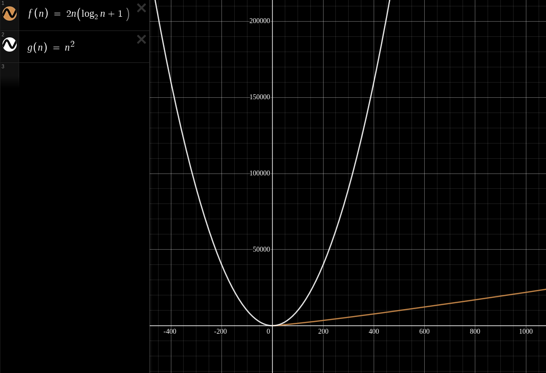
If we do a naive sequential search of the lists to find a solution , the computational work needed find that solution remains roughly the same (gargantuan) regardless of how many lists we have. At best, searching only two lists of length , we’re talking a complexity of , which for secp256k1 is about computations. By the time we find the solution, the sun will have exploded, heat death of the universe yadda yadda - you know the rest.

We’re assuming is cryptographically secure, so can’t rely on hash collisions, preimage attacks or other cheat-codes like that.

So what’s a cypherpunk to do?

A classic trick of algorithmic efficiency is to break down a complex task into smaller and simpler ones.

It is evidently too difficult to find a solution when hashes are all evenly distributed among . If is very large, the number of combinations we’d need to check would be absurd.

It would be easier if we only had to look for solutions distributed among a smaller range than . Because the lower-bound of the list length is determined by the size of the range we’re searching within (i.e. ), we can make it easier to find a solution if we can find a clever way to reduce the size of that range.

Let’s explore a particular example of Wagner’s Algorithm where (eight lists) and we want to find hashes from each list such that they all sum to when taken mod .

Why sum to instead of ? This makes Wagner’s algorithm much easier to execute, and we can do so without loss of generality: One list is modified by subtracting from each random hash in . This results in the correct set of solution hashes summing to .

We will build a binary tree, and break the problem into smaller chunks at each distinct height of the tree by merging lists together while preserving important properties in child lists, and maintaining pointers back to the hashes in the original lists.

After building the final root node list , we should expect to find at least one solution, and we can follow the pointers back up the tree to find the original hashes which created that solution.

Merging The Leaves

Perhaps we could merge two leaf lists into list at height while maintaining the same list length, but with elements distributed across a smaller domain using some yet-to-be-defined operation .

When merging two parent lists into a child list , we want to capture two important properties in the child list:

1. Elements in the child list should be distributed across a significantly smaller range of possible values than the elements in the parent lists.
2. Elements in the child list should be the sum of two elements from the parent lists. Each child list element should maintain pointers to the two elements in the parent lists which created them.

Our approach to merging will be to iterate through every combination of candidate elements from both lists, and test to see if their sum falls within a certain range around zero, wrapping modulo . At the height , the range will be a certain size, and at we will shrink the range to further reduce the necessary domain.

How big should that range be?

Let’s parameterize the filter range for height as some interval wrapping around zero modulo .

We don’t know what that interval is yet, but we can deduce what it should be.

Assume the two leaf lists each have the same length . We want to expect the child list to also have length so that when we apply this operation for future children of , we still only need to search approximately possibilities each time.

Since both parent lists have length , we have combinations between them. To maintain approximately the same length in the child list we need the probability of the sum of two randomly sampled elements falling into the range to be exactly .

If we independently roll this probability once for each unique pair in lists , we would have rolled it exactly times. Due to Linearity of Expectation, we should expect about pairs from the parent lists to filter down into the child list. This gives us exactly what we want: The child list will contain about elements.

We already know that the probability of two elements randomly sampled from summing to a particular number modulo is . But what if, instead of summing to a single number, we ask whether falls into a range of size ?

Intuitively it should make sense that the probability then becomes , since we have chances instead of chance for the random roll of the -sided die to land where we want it to.

We can use this relationship to compute how large the initial filter range needs to be in terms of and .

Booyah! A filter range of size at height will result in our desired filter probability , and thus our desired expected child list length .

For a range of size around , we should set

The range will thus have size .

To rephrase more succinctly: If we make random rolls of an -sided die (i.e. random sums modulo ), we should expect around of those rolls to land in the range , thus ending up in the child list .

The elements in the merged child list have an important distinctive property: They are now distributed randomly throughout , instead of throughout . This range has size - much smaller than .

Furthermore, if we add together any two elements sampled from , their sum will fall within the range : a range which is predictable and easy to work with.

Merging the Children

What about for other heights?

When we merge the lists , we will be working with lists of the same expected length , but with elements distributed among a much smaller domain: . This allows us to further reduce the filter range for height , and for other heights as well.

In general, if we want to expect elements in each merged list, we want each each filter range be about times the size of the previous range .

This gives us a generalized formula for the operator.

By repeating this procedure, merging lists in a tree-like pattern, we can gradually reduce the domain among which elements in each merged list are distributed.

Height	Filter Range Size
…	…

Remember as well that for every pair of elements whose sum falls into the filter range, we must maintain two pointers from back to its parent elements . This is required for Carol to be able to find the original candidate hashes which were summed to produce the final output solution. If , then all ancestor elements which were summed to form and will also themselves sum to .

If a merge operation ever outputs an empty list, this is a failure condition and it means we need to retrace our steps, starting over with new randomly generated leaf lists. If we merge an empty list with a non-empty list , the output will always be empty, since there are no pairs of elements possible between and .

Finding the Solution

Remember our goal is not just to shrink the domain but to find a tangible solution. Thankfully, as we cinch the domain of elements closer around zero, we become exponentially more likely to find solutions. By merging lists, we are reducing the number of lists - thus reducing the number of permutations we have to check - but also we are increasing the probability that any set of elements from lists of a given height will sum to zero mod .

We will ultimately need to perform a different operation to create the final root list . This operation will not involve a filter range. We instead perform a set intersection operation to see if the penultimate lists and share any elements which sum to zero mod .

The obvious way to do this is to define the operation directly (but less efficiently) by iterating through every combination of the operand lists and , looking for sums of zero.

More efficiently, we could perform as an intersection of the lists and , where indicates each element in the list is negated mod . This allows us to use faster algorithms like a hash-intersection, with time complexity .

Consider the following lists:

If , we want to contain only elements created by summing to zero mod . This would obviously be from and from , because .

Returning to our example, we could describe the whole algorithm’s operations as follows.

For efficiency, we don’t actually want to evaluate the whole tree top-to-bottom like this, because doing so would require that we keep unnecessary lists in memory during the procedure, which might be expensive if those lists are large, or if there are lots of lists. It would be better if we only load the lists into memory (or generate them) when needed.

Thanks to the tree structure of the algorithm, we can evaluate the merging operations in a deferred sequence to reduce memory requirements. We could discard the elements of parent lists if they are no longer referenced by the child lists they are merged into.

For our example, the merging operations would be computed in this sequence:

Leaf lists like and would only be generated once needed. Once a list is no longer needed, we can discard it, keeping only references to elements which were passed down to merged child lists.

This way, we don’t have to store so much data in memory at once. Instead we only have to store a maximum of 4 lists at a time in this example: two in storage and two in working memory (to perform merge operations). For larger values of we would need more storage, but still only two lists need to exist in working memory at a time.

List Length

We still have yet to fully understand how to choose our list length , so let’s flesh that out.

When we build the root list , want both penultimate parent lists to contain elements distributed among a range whose size is around . This way, with permutations (on average) between , we can expect about solutions (on average) when joining to make the root list.

The height of the penultimate lists will be , i.e. the last height before the root node. For , that is height .

This makes sense for our example:

Thus, we want . But wait, didn’t we already define the size of any given filter range? We did!

And we can make use of that to compute what should be!

In general, we can choose the list length for number of lists modulo , since we will always want the size of the penultimate range to be .

In english, should be the -th root of . This ensures all the probabilities and expectations we’ve set up will work out as we planned, and we should hopefully get a solution out once all the lists have been merged.

Full Description

Above I’ve tried to walk through the steps of Wagner’s Algorithm in detail, justifying each step in an attempt to make it seem more approachable.

In this section, I’ll provide a bare description of the algorithm itself applied to InsecureMuSig, and omit the full reasoning behind each operation.

1. Fix the modulus and the desired sum .

2. Choose , which describes how many lists we want to search, and how many concurrent signing sessions Carol will need to open with Alice and Bob.

3. Compute the list length .

4. Define the list-generation procedure for lists , by sampling randomized inputs per list.

For the last leaf list , subtract from each of its elements.

For better memory efficiency, these lists should only be generated once they are needed. Each hash must contain a pointer to the curve point which was used to create it.

5. Define the merge operation for a given height . This operator merges two lists into a new list at height by summing each combination of two elements, one from each list, modulo and including the sum in its output list if the sum falls within an inclusive range , wrapping modulo .

Every element in the output list must contain two pointers to the parent elements which were summed to create .

6. Define the join operation which will be used to construct the final root list at the maximum tree height . This operator returns a list composed solely of zeros which also have pointers to the parent elements which were summed to create them.

7. Begin merging lists.

• Start by generating the first two leaf lists and , and merge them as at height .
• Generate lists and . Merge them as .
• Merge these two lists at height .
• Generate new lists and .

Continue in this fashion, proceeding to the next height whenever possible, generating new leaf lists and merging them as required, until we have the two penultimate lists at height .

If a merge operation ever results in an empty list, discard this branch of the tree and start over with freshly generated leaf lists.

8. Join the penultimate lists and with the join operator .

If is empty, start over again with freshly generated leaf lists.

9. If contains at least one element, follow its pointers back up the tree to the hashes in the leaf lists. The result will be a set of hashes such that .

10. Follow the pointers from the leaf elements to find the curve points which were hashed to construct each element. Since the last leaf element was constructed by subtracting from the actual challenge, this means the set of nonce points will result in signature challenges which sum to .

11. Carol can now provide rogue nonces to Alice and Bob so that are used as the aggregate nonces in each of the signing sessions, as discussed before.

Performance

Let’s analyze the computational complexity of Wagner’s Algorithm.

• At each list-merging operation (), we must perform simple addition operations.
• At the root node at height , we perform a join operation which uses computations. These operations are insignificant next to the rest of the computations though, so we can safely ignore them.
• We must perform merging operations at height , then merging operations at height , then operations at , and so on.
• This means we perform merges, for a total of simple addition operations.

The sequence can be rewritten as the sum of a finite geometric series:

The sum of a finite geometric series starting at with ratio over iterations is . Therefore:

Because :

A quick sanity check and our formula seems to work:

Thus in total, we perform simple operations, which make up the bulk of the computational work in the algorithm.

Optimizations

There’s an easy optimization which boosts the speed of Wagner’s Algorithm by at least one order of magnitude.

The bulk of the work occurs when adding together every combination of elements between two lists of length , and filtering the sums based on a range modulo . The merging operation as I’ve described it above would look something like this in Python.

def merge(L1, L2):
  sums = []
  a, b = filter_range(height)
  for e1 in L1:
    for e2 in L2:
      z = (e1 + e2) % n
      if z >= a or z <= b:
        sums.append(z)
  return sums

The complexity thereof is , because as written, it appears we have to test every possible combination of elements, but this needn’t be so.

Remember that and are simple collections of numbers. We can restructure them however we want to improve efficiency and save work. There exist all manners of data structures for doing this.

One option would be to sort the list prior to iterating through . For every we draw from , we now have the benefit of working with a sorted .

Observe how for any given , there is only a specific range of values which can be, such that . Namely:

Any values in outside the range need not be checked at all, because we know for certain that they will never sum with to a value in .

If is sorted, we can use a binary search to quickly ( complexity) find the location in where elements close to would be sorted. We then iterate through those elements in , adding them to the new merged child list until we reach an element larger than , at which point we can halt our search of , and continue to the next element in .

As an example, consider a case where:

We are merging two lists like so:

• First, we loop through and encounter the element .
  • Compute the minimum viable value for as .
  • Since is sorted, we can binary search it to quickly find where we could expect to find if it existed in . It would be at the very end of though, so we wrap around to the beginning of and begin our search there at .
  • , which does not fall into the range . We can now discontinue our search for a partner sum for . This checks out, because indeed there is no number which would sum with such that .
• Continuing our loop through , we encounter the element .
  • Compute the minimum viable value for as .
  • Binary search to find where would sort into . We find the index for the next highest value in : .
  • Beginning our search here, we find that which does fall within . We add to the output list and continue looping forward through .
  • We hit the end of , but once again we wrap around to the beginning of . We encounter the element .
  • does not fall within the filter range. We discontinue the loop here and move on to the next element of . Again this checks out, because no can provide .

In Python, this might look something like so:

from bisect import bisect_left

def fast_merge(L1, L2):
  sums = []
  a, b = filter_range(height)
  L2 = sorted(L2)

  for e1 in L1:
    min_index = bisect_left(L2, (a - e1) % n)
    index = min_index
    while index < min_index + len(L2):
      e2 = L2[index % len(L2)]
      z = (e1 + e2) % n
      if z >= a or z <= b:
        sums.append(Lineage(z, e1, e2))
      else:
        break # no more useful elements to be found.
      index += 1

  return sums

This new merge operation has significantly lower complexity.

• It requires one sorting operation per merge, which can be done in time with an algorithm such as heapsort, quicksort or merge-sort.
• Once has been sorted, we loop through for a total of iterations.
• On each iteration, we perform a binary search of in time. We then add an average of 1 element to the output list (since we expect to have elements), and also perform one extra check which tells us when we run out of useful elements in .

In total, our new merge operation algorithm requires

computations. It runs in time.

This is a big improvement over the complexity for the naive sequential algorithm. For lists of small size, there is barely a difference, but the larger becomes, the greater the efficiency savings. For all , the binary-searching algorithm takes the cake.

To put this into perspective, merging two lists of length we’d be doing about 91 times more work with the sequential merge algorithm.

Since we are performing merges in total, the whole algorithm requires operations.

Choosing

If we fix , note that the more lists we have - i.e. the higher is - the fewer elements we need in each list, because . For instance, with secp256k1’s , then with , we need hashes per list. With 128 lists () we need only hashes per list to be able to find a solution with Wagner’s Algorithm.

Does fewer elements per list result in fewer computations overall? Is there some ideal number of lists which optimizes the amount of computation required to find a solution? In our case, we can set to whatever we want within reason - as long as Carol can effectively manage concurrent signing sessions with Alice and Bob.

The total work we need to do is . If you wanted to be a fancy-pants, you could take the derivative of this expression with respect to , and find out exactly how many lists would be most efficient for any given value of .

But however nerdy I may be, I am also adverse to pointless effort. It would be much easier to simply guess and check every plausible value of for a given . Since we only want values of which are powers of two, such a test should be very simple and fast.

from math import log2, inf

# secp256k1 curve order
n = 0xFFFFFFFFFFFFFFFFFFFFFFFFFFFFFFFEBAAEDCE6AF48A03BBFD25E8CD0364141

min_computations = inf
best_k = 1

for log_k in range(2, 32):
  k = 2 ** log_k
  lamda = n ** (1 / (1 + log_k))
  computations = round((k - 2) * (2 * lamda * (log2(lamda) + 1)))

  change = computations - min_computations
  print(
    "k =% 8d; computations required:% 30d; change: %+.2f%%" %
    (k, computations, 100*change/min_computations)
  )

  if computations < min_computations:
    min_computations = computations
    best_k = k
  else:
    break

print()
print("Best is k = %d = 2^%d" % (best_k, log2(best_k)))

k =       4; computations required: 16831834955285952201643524096; change: +nan%
k =       8; computations required:       14388460377493450260480; change: -100.00%
k =      16; computations required:           3780631184960625152; change: -99.97%
k =      32; computations required:             18291434784828656; change: -99.52%
k =      64; computations required:               475747350059814; change: -97.40%
k =     128; computations required:                35716948033536; change: -92.49%
k =     256; computations required:                 5463841149033; change: -84.70%
k =     512; computations required:                 1379906617598; change: -74.74%
k =    1024; computations required:                  502792114295; change: -63.56%
k =    2048; computations required:                  241469572845; change: -51.97%
k =    4096; computations required:                  143536403739; change: -40.56%
k =    8192; computations required:                  100948092745; change: -29.67%
k =   16384; computations required:                   81255644943; change: -19.51%
k =   32768; computations required:                   73009987584; change: -10.15%
k =   65536; computations required:                   71840273971; change: -1.60%
k =  131072; computations required:                   76265276072; change: +6.16%

Best is k = 65536 = 2^16

Looks like for secp256k1, the best case for computation time of Wagner’s Algorithm is for a total of lists. Notice that beyond a point we start to see diminishing returns as we further double .

Realistically, Carol may want to set somewhere between and . Below lists, Carol would lose out on orders of magnitude of efficiency savings. Above lists, it would become impractical for Carol to execute so many concurrent signing sessions with Alice and Bob, and she wouldn’t even be gaining any more computational efficiency savings by taking the risk.

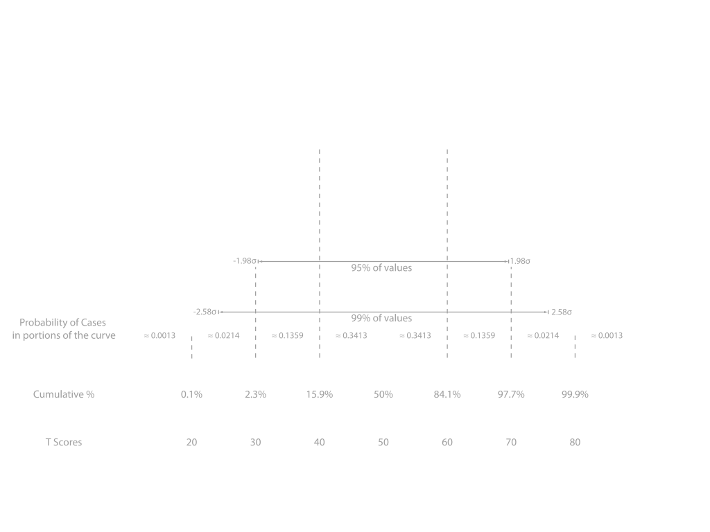
Normal Distributions

There is one odd detail of Wagner’s Algorithm which still mystifies me.

If we sample two random elements from lists at height and add them together modulo , those sums will form a normal distribution (AKA a bell curve) among a range which is double the size of , and centered on .

This is because the filter range is less than half the size of , so when we add two elements from together, their sum could be at most , and at minimum .

Thus, for any pair randomly sampled from , the distribution of their sum will not be a perfectly random -sided die as we had at . With each sum we are rolling a weighted probability, where sums closer to are more likely to occur, since there are more pairs of numbers in which sum to values numbers to .

To better understand this, imagine a smaller-scale hypothetical example where . If we sample two random values from and sum them, we will get a normal distribution. Provided each value in is equally likely to be sampled, we can arrange two copies of in a grid and visually see which sums are most common.

+	-5	-4	-3	-2	-1	0	1	2	3	4
-5	-10	-9	-8	-7	-6	-5	-4	-3	-2	-1
-4	-9	-8	-7	-6	-5	-4	-3	-2	-1	0
-3	-8	-7	-6	-5	-4	-3	-2	-1	0	1
-2	-7	-6	-5	-4	-3	-2	-1	0	1	2
-1	-6	-5	-4	-3	-2	-1	0	1	2	3
0	-5	-4	-3	-2	-1	0	1	2	3	4
1	-4	-3	-2	-1	0	1	2	3	4	5
2	-3	-2	-1	0	1	2	3	4	5	6
3	-2	-1	0	1	2	3	4	5	6	7
4	-1	0	1	2	3	4	5	6	7	8

As you can see, is the most common sum. The same will also be true of our lists of hashes. The sum of two elements randomly sampled from will also tend to be clustered more densely around , since we defined the range to be centered at .

Notably this does change the probability math when computing how to define our next filter range . We wanted to define the interval such that the probability of falling into is exactly .

Strangely however, Wagner’s original paper makes no mention of this normal distribution. Wagner only illustrates the generalized form of his algorithm for , where this distribution never occurs, because never rises above .

We can also apply the tree algorithm to the group where is arbitrary. Let denote the interval of elements between a and b (wrapping modulo m), and define the join operation to represent the solutions to with . Then we may solve a 4-sum problem over by computing where and . In general, one can adapt the -tree algorithm to work in by replacing each operator with , and this will let us solve -sum problems modulo about as quickly as we can for xor.

In his paper, Wagner focused on solving what he dubbed the -sum problem: finding numbers from randomly generated lists which sum to zero. However he was clearly more focused on finding binary numbers which XOR to zero, rather than on additive groups of integers modulo (or , as Wagner used in the above excerpt). It’s possible he never considered this consequence of the generalization of his algorithm, or perhaps he knew but realized it was inconsequential and so omitted it from his paper.

Peculiarly, Wagner’s Algorithm still seems to work for large values of , so the normal distribution doesn’t appear to have a significant effect on the probabilities involved. I spent some time trying to work out the exact probabilities at , but once I realized the change was negligible, I abandoned that line of investigation.

Implementation

To prove to myself that this absurd-seeming procedure actually works, I wrote up a pure Python implementation of Wagner’s Algorithm. Click here to view the code on Github.

You can install and use it with pip install wagner.

import random
import hashlib
import wagner


def hashfunc(r, n, index):
  r_bytes = r.to_bytes((int.bit_length(n) + 7) // 8, 'big')
  preimage = r_bytes + index.to_bytes(16, 'big')
  h = hashlib.sha1(preimage).digest()
  return int.from_bytes(h, 'big') % n


def generator(n, index):
  r = random.randrange(0, n)
  return wagner.Lineage(hashfunc(r, n, index), r)


if __name__ == "__main__":
  n = 2 ** 128
  preimages = wagner.solve(n, 888, generator=generator)
  print(sum(hashfunc(r, n, index) for index, r in enumerate(preimages)) % n) # -> 888

My code demonstrates that although the attack is plausible, it is still very hard to pull off. Not to disparage my performance optimizations, but the procedure is quite slow for large values of . The practical limit to compute a solution in a reasonable amount of time, at least on my current machine, is - much smaller than secp256k1’s .

Beyond this, the procedure is too slow to execute a real-world attack. After opening her signing sessions, Carol cannot wait too long to compute the points . She needs to compute those points relatively quickly so she can determine which rogue nonces to supply to Alice and Bob. If Carol takes too long, Alice and Bob may have given up on the signing sessions, or even realized what Carol is up to.

However, simply because my code does not compute solutions fast enough doesn’t mean the attack is infeasible. There exist many much stronger computers out there, and I have barely scratched the surface of the possible optimizations one can make to Wagner’s Algorithm. Not to mention I wrote my implementation in one of the slowest programming languages in town, and made no attempts whatsoever at parallelization. With enough rented cloud computing power, a faster language like C or Rust, and a cleverly optimized implementation, it would certainly be plausible to execute this attack.

Conclusion

Thankfully, the whole attack has been made obsolete against the real MuSig, due to the nonce commitment round which was introduced in the updated MuSig protocol. Without the option to choose rogue nonces, Carol cannot control the challenges.

However, as Blockstream’s Jonas Nick writes, Wagner’s Attack is definitely still applicable to MuSig in some edgecases though. It pays for devs to really understand how this attack works, so that hopefully we can avoid reintroducing the same vulnerability when creating new protocols or when optimizing existing systems.

The subtle math behind the attack is fascinating. It goes to show that however experienced one might be, the true test of a cryptosystem occurs when it is exposed to a critical and observant community. It is absolutely essential for experts to attack each other’s systems. There’s simply no way for any one person (or even a group of people) to collectively hold in their mind all the myriad ways their system could be attacked.

In cryptography, a solid proof is like a well-forged sword… but rigorous peer review is the grindstone, and time is the foot which effects the sharpening.

Sources

• On the Security of Two-Round Multi-Signatures - Drijvers et al
• A Generalized Birthday Problem - David Wagner
• Insecure Shortcuts in MuSig - Blockstream
• https://bitcoin.stackexchange.com/questions/91534/musig-signature-interactivity
• Birthday Attack - Wikipedia